Archives:Simulation of Oil Reserves on a Digital Computer

Copyright@1964 Dr. E. L. Dougherty and H. C. Mitchell

Introduction

Petroleum reservoir engineering may be defined as that branch of applied science which strives to understand the mechanics affecting petroleum reservoirs and petroleum production, and to apply that understanding to the efficient operation of petroleum reservoirs. During recent years, this branch of engineering has experienced tremendous growth in both depth and scope. Increased demand by our society for energy, increasing difficulty in discovering major quantities of domestic petroleum, and greater governmental concern, both domestic and foreign, for maximizing utilization of national resources, have added to the natural impetus of scientific curiosity in this field. The development of digital computers has contributed greatly to advancing this branch of applied science because it provided a possible means for performing the enormous volume of calculations required to solve complex reservoir engineering problems.

In this paper, we will concern ourselves with the application of models to oil reservoirs. Models may be either physical or mathematical analogs, and may represent the behavior of individual wells or large reservoir-aquifer systems. A well model is used to study pressure and saturation behavior in the vicinity of the well bore. In a reservoir model, the detailed behavior around wells is not calculated, but the gross effects of wells are included. Pressure and saturation behavior is studied over the entire petroleum reservoir and surrounding aquifer, or over several petroleum reservoirs interacting through a common aquifer.

Historically, the case history approach was the first method used to predict reservoir behavior. From a knowledge of the performance of a depleted or nearly depleted oil reservoir with properties similar to the reservoir to be studied, forecasts of the performance of the new reservoir are made. To the extent that the two reservoirs and their operating conditions are alike, accurate predictions of future perfor¬mance can be made. Because it is seldom possible to find two nearly identical reservoirs with identical operating conditions, this approach is severely limited.

The first widely employed technique for predicting reservoir per¬formance which used the concept of a mathematical model was' that of material balance. This approach was first suggested by Coleman in 19291 but did not develop into a really useful tool until the mid-thirties following the work of Schilthuis2and Tarner3. The material balance approach utilizes the concept of conservation of matter and thermodynamic relationships but does not consider flow dynamics; i.e., the reservoir is treated without regard to spatial arrangement. Al¬though this development was a major contribution and is still widely used today, inability to consider hydro- dynamical effects, in many cases, is a decided drawback.

The development in the forties of relative permeability theory as a modification of Darcy's Law to describe two-phase flow resulted in the basic equations of motion for oil, gas, and water. These equations in their general form represent a fairly rigorous mathe¬matical model of reservoir-aquifer systems. Some assumptions regar¬ding the thermodynamic system and the reservoir rock material are still necessary, however, in developing these equations. In varying degrees of simplification, these equations form the basis for most mathematical reservoir modeling today. If the process does not vary with time, steady-state equations result. These equations find use in reservoir modeling, especially in certain problems concerned with calculating areal sweep efficiency. In most cases the processes vary with time, so that the more complex transient equations are more often encountered in reservoir modeling. In this paper we will confine our attention to reservoir models rep¬resented by unsteady-state equations. The basic aim in reservoir modeling is to match calculated pres¬sures to observed field pressures through suitable adjustment of certain parameters in the model. When a satisfactory history match is obtained, the model is used to predict future pressure-production performance resulting from anticipated production schedules. Thus, via the case-study approach an approximation to an optimum production schedule can be obtained.

One Dimensional Models

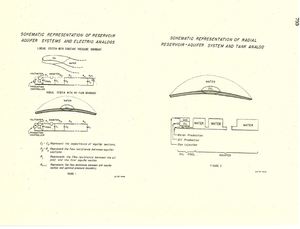
The partial differential equations describing transient flow of fluids in oil reservoirs are quite complex in their general form. As a result, they are not tractable by analytic methods unless simplifying assumptions are made. However, the rapid development of automatic sequenced digital computers and advances in numerical techniques during the past two decades have provided a- means for solving the general equations. Because the techniques are not simple, obtaining solutions in a reasonable length of time of the more general problem requires use of the largest and fastest digital computers. For certain types of problems, one dimensional representation is satisfactory. This is the case when only limited reservoir data are available or when only gross information about the behavior of the reservoir and its surrounding aquifer are required. Studies of this type have been performed in the past with electrical models. Figure 1 shows a schematic representation of two oil field-aquifer systems and their electrical RC analogs. The condensers represent the com-pressibility of the several parts of the system and the resistors represent the single phase flow resistance of the system.

An improved model is obtained if compressibility is allowed to vary with pressure and the effects of two phase flow and gas solubi¬lity are considered. This can be done by numerically solving a math¬ematical analog with the aid of digital computers. Figure 2 depicts the representation of a radial reservoir-aquifer system as a series of tanks. The tanks may contain oil, gas, water or combinations of the three. For the radial system shown, the tanks are annular rings so that their volume increases directly with distance from the oil tank. The pipes connecting the tanks represent the resistance to flow afforded by spatial considerations in the real system. Because the cross-sectional area between rings increases with distance from the center of the radial system, the resistance to flow between rings decreases outwardly. This is reflected in the size of the pipes in Figure 2. With this type of model, it is possible to treat both one and two phase flow between tanks. If the physical system being modeled so dictates, the oil reservoir may be represented by more than one tank and fluid flow between oil field tanks considered. In order to simplify further discussion let us assume all gas and oil are confined to one tank. This eliminates consideration of permea¬bility varying with saturation.

Two Dimensional Models - Single Phase Flow

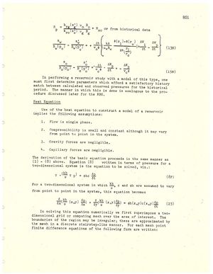
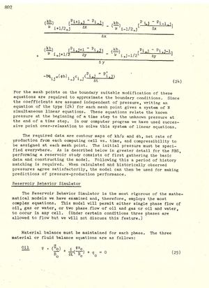
Single phase flow problems with nearly constant compressibility, for which one dimensional or quasi-one dimensional models do not pre¬sent sufficient spatial details, may he treated by a suitable repre¬sentation of the two dimensional heat flow equation. This was done by Bruce4 in 1943 with an electrical RC network analyzer, a two dimen¬sional network of resistors and condensers similar in concert to the one dimensional electrical models shown in Figure 1. The two dimensional heat flow equation with spatially varying co¬efficients' can also be readily solved numerically. There are certain inherent advantages to the digital approach. Because of the general nature of the computations which can be performed on a digital computer, it is possible to mechanize great deal of the enormous amount of data processing required in a reservoir study. Tables of all of the perti¬nent data such as production and injection volumes, formation permea¬bility and porosity are stored on magnetic tape and/or punched cards and can be automatically called in by the program as required. Considerable flexibility with regard to output information can also be provided. Pressures can be printed in tabular form and the program can be made to generate contour maps of these data.

An additional advantage of the digital simulator is the relative ease with which modifications can be made to existing models or with which new models of the fields can be generated. Furthermore, the program is a general tool which can be processed at any of a large number of digital computer installations. Thus, different models could be studied simultaneously at different installations if this should prove desirable.

Two Dimensional Models - The Multiphase Flow

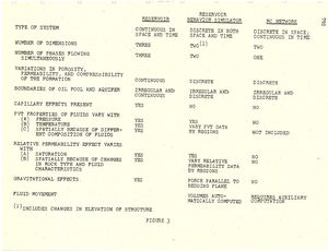
More advanced digital reservoir simulators have been developed by researchers in the petroleum industry to treat two and three dimension¬al flow including the effects of two phase flow, gravity and time vary¬ing saturation and compressibility. We shall describe in detail one such model which treats two dimensional flow; we shall henceforth refer to the system of computer programs comprising our system as the Reservoir Behavior Simulator (RBS). 15 There is no electrical analog equivalent to the RBS; the RC network analyzer is the closest such device. Figure 3, which presents a comparison of the treatment affor¬ded by these two modes of simulation, illustrates the inherent super¬iority of digital simulators.

Geometry of Model

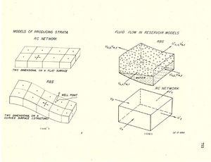
Conceptually, in the RBS, the producing strata is considered to be a curved surface passing through the midpoint of the actual formation. Thickness of the strata is included in computing capacity and conduc¬tivity, but no flow is allowed perpendicular to this surface (Figure 4). Thus, the conditions predicted by the RBS must be considered to be the average of those in the actual reservoir, the average being taken across a section perpendicular to the bedding plane. The fact that the surface is curved allows incorporation of variations in ele¬vation of the formation and makes it possible to take into account the effect of the component of gravity acting parallel to the bedding plane. Also shown on the figure is the RC network representation which considers the reservoir to be planar.

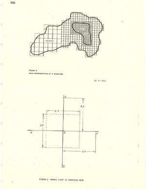
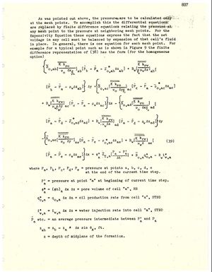
These diagrams call to attention the fact that in both models the reservoir is subdivided into discrete blocks. Pressures and satura¬tions are defined only at the centers of these blocks, i.e., at the mesh points. Each mesh point is assigned the fluid capacity of the surrounding block. The values of permeability which appear in the equations relating flow between adjacent mesh points are average values which represent the conductivity of the rock separating these points. If the location of a well does not coincide with a mesh point, the production from that well must be allocated to the surrounding points. Techniques for performing this allocation which will give a good approximation to actual field behavior have been developed for the RBS.

Fluid Flow in Model

The manner in which fluid flow is handled in the RBS and .Rc network is represented pictorially in Figure 5. In each case, fluid enters or leaves through all four faces of the computing cell. In the RC analy¬zer the flow is considered to be single phase, either water or oil. On the other hand, the RBS can handle either single-phase or two-phase flow. In computing saturation changes in the two-phase flow region, two options are available in the RBS. The segregated option considers the fluids to be segregated within each cell; the homogeneous option treats the two phases as if they were uniformly mixed throughout the cell. The segregated option is represented in Figure 5.

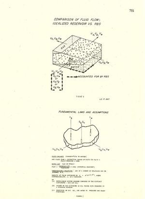
Figure 6 calls attention to the facts that across a given trans¬verse section of the actual reservoir three phases may be flowing simultaneously and. that the body force of gravity is acting verti¬cally on every particle of fluid. Each phase has in general three velocity components, one perpendicular and two parallel to the bedding plane. In the RBS, only the component of gravity and the two velocity components parallel to the bedding plane are considered; the latter are really averages over the cross-section perpendicular to the bedding plane.

Development of the Equations

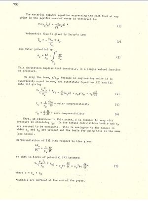
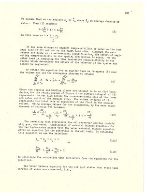
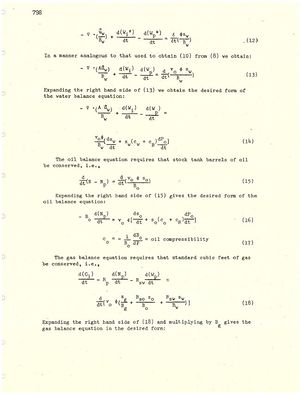
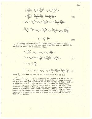
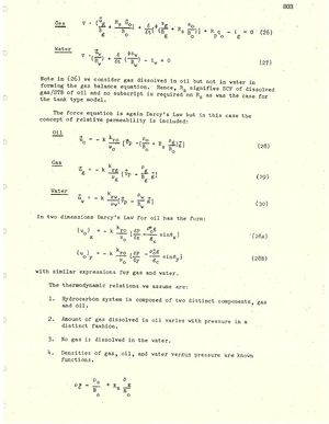
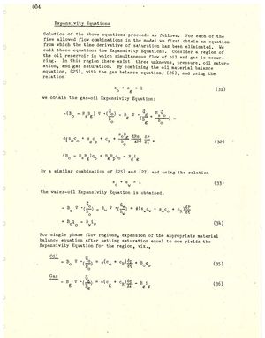
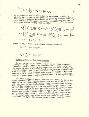
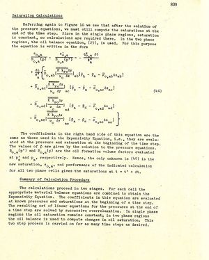
All reservoir simulators are based upon the three fundamental laws or assumptions depicted in Figure 7. The material balance equations are based upon the law of conservation of matter and state that the mass of each fluid phase must be conserved. The second relationship is the law of force which for nonturbulent fluid flow through porous media is simply Darcy's Law. The third relationship defines the thermo¬dynamic behavior of the system. Depending upon the system and the accuracy desired in representing the system, any of a number of thermo¬dynamic relations may be assumed. The basic equations for any reser¬voir simulator are developed from these fundamental laws. We will show how this is done for the following models:

One dimensional with pressure dependent compressibility and gas solubility (Tank Type).
Two dimensional with single phase flow and small constant compressibility (Heat Equation).
Two dimensional with saturation dependent permeability, pressure dependent compressibility and gas solubility, and including gravitational effects (Reservoir Behavior Simulator).

Tank Type

For the tank type model wherein water-is the only fluid moving from tank to tank, the equation of motion for single phase flow of water' must be solved simultaneously with a gas, oil and water material balance equation for the oil tank.

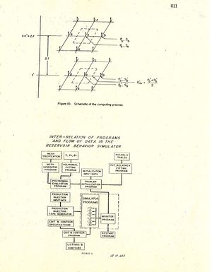
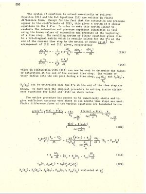
In the field of numerical methods the formulation is called "implicit" with regard to the pressure and "explicit" with regard to saturation. Owing to the use of an "explicit method" for saturation, the method is subject to a stability condition which limits the size of the permissible time step. The stability condition is difficult to state precisely owing to the method by which mobilities are computed. However, one can state that it is probably necessary to keep the time steps small enough so that the amount of fluid flowing across each cell face during a time step is less than some fraction of the pore volume of a cell. Figure 11 illustrates the inter-relation of the programs comprising ‘the Reservoir Behavior Simulator and the flow of information from one program to another. There are approximately twenty-five computer programs in this suite of programs that are commonly used. These have been programmed for a 32K IBM 7090. The programs may be roughly broken into three groups, the preprocessors, the equation solvers, and the post processors. The mesh generator, initialization, and PVT relative permeability programs are examples of the preproces¬sors. The simulator programs 1 through 6-are the equation solvers, and the edit and contour programs are the post processors. It is well to emphasize again the value of the programs which perform essentially auxiliary functions. The ability to automatically process input data and obtain results in a wide variety of forms is of prime importance.

Example

To gain a better understanding of the types of problems we are solving with the Reservoir Behavior Simulator and the steps involved let us consider a hypothetical oil reservoir in a large aquifer. The reservoir has been produced for about six years. We would like to know what will happen to pressure and saturation in the reservoir if we produce at a rate corresponding to our best estimate of demand. Let us call this Case A. We would also like to know what will happen if we produce at a rate above forecasted demands, Case B. We are also interested in studying the effect of a "crash" production rate which would require drilling additional wells, Case C.

Computing Mesh

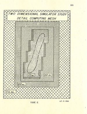
Let us assume geological data indicate the oil field is located in the middle of an aquifer with dimensions approximately 25 x 30 miles. The aquifer is assumed to pim.eh out forming no-flow boundaries, thus establishing the boundary conditions for our model. Once the limits of the region to be covered. have been defined, the desired number of mesh points is allocated to the interior of the region. For this model we used 1200 mesh points. For reasons discussed above we used a square mesh 0.2 x 0.2 mile in the oil pool and increased this to a square 3.2 mile mesh in the outer limits of the aquifer.

Figure 12 shows the central portion of the computing mesh for our hypothetical oil field. The outer limits are not shown because of the large size of the model. Having mesh size change by a factor of two simplifies the computations. The small areas outlined between the 0.2 and 0.11 mile mesh indicate that either a 0.2 x 0.4 or 0.4 x 0.2 mile rectangular mesh was required to make the mesh size changes come out properly.

Once the general layout of the computing mesh is defined by hand, the necessary data are fed into the computer and a program generates the detailed computing mesh. It assigns points wherever these are required, numbers them sequentially and generates a magnetic tape containing the point number and its coordinates. With this program the maximum number of mesh points is 3000.

Reservoir Data

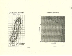
The values of permeability-thickness, porosity-thickness and structural elevation are usually given in the form of contour maps such as is shown for permeability-thickness in Figure 13 for our example study. This map is used to compute fluid conductivity and the porosity-thickness to compute fluid capacity of the model. Structural elevation data must be provided, because the effects of gravity parallel to the mid-plane of the formation are treated.

There are two methods for introducing these three sets of data into the RBS. One, referred to in Figure 11 as polynomial fitting, consists of fitting a rational function of Legendre polynomials in a least square sense to values of any one of the three structural properties taken uniformly from the contours in a given rectangular region. More than one set of polynomials may be used to describe a given structural property throughout the model. Since the mesh point tape contains the coordinates of the mesh points, and since this same coordinate system is used in the fitting polynomials, the RBS can determine the desired structural value at any point in the model. This approach has proven unwieldy.

The second method uses a data file constructed by manually reading values from the maps at the mesh points. Since this process is performed only once it is not too burdensome, and is the technique we ordinarily use.

For the hydrocarbon fluids, tables of oil viscosity, gas viscosity, oil formation volume factor, gas formation volume factor, and solution gas-oil ratio versus pressure are required. Figure 14 illustrates the oil formation volume factor data. The fluid data are entered into the program by fitting equations of the form y = a0 + a1p + a2p2 through sections of each curve, the number of sections being arbitrary. When the program needs values for these variables, they are obtained by computing them from the appropriate equation.

Relative permeability data for both the gas-oil system and the water-oil system are required. These data are handled within the machine in the same fashion as the PVT data, except that the indepen¬dent variable in this case is oil saturation. As many as 20 different relative permeability regions using different kg./k0 and kw/ko curves can be used in the same computing model. Both the PVT and relative permeability data are based upon laboratory measurements of field samples. In addition to detailed data for the hydrocarbon fluids, data are required for formation volume factor of water as a function of pressure and viscosity of water. Compressibility of the rock is also needed.

In addition, it is necessary to provide the RBS with tables of cumulative production, gas injection, and water injection. The data in the present model include only oil production and water injection. In assigning initial pressures, the entire model was assumed to have been in hydrostatic equilibrium at the start of operations. Initial oil saturations were assigned, neglecting connate water saturation, in such a fashion as to maintain the proper volume of oil in place. Miscellaneous control data for the several programs complete the data requirements.

History Matching

Having assembled the necessary data in the proper form and com¬pleted the preprocessing, one is ready to begin history matching. This phase of the study will consist of several computer runs during which various parameters are adjusted to bring calculated pressures into agreement with observed pressures. The proper parameter adjust¬ment is not a straightforward operation. It is often lengthy and expensive. Work is now under way to systemize this process using computers.

Results of Study

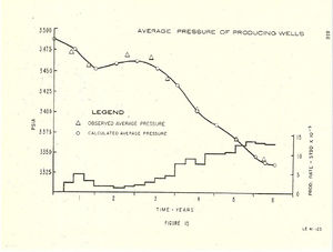
Figure 15 shows average pressures for production wells versus time, both observed values and calculated values. This exhibit shows the quality of the final history match. The average pressures used in this figure were obtained by averaging values from all wells except certain wells with abnormal performance. It will be noted that the calculated average pressure curve follows the observed pressure data within 2-5 psi over the last three years of history. During year 2 and 3 the greatest deviation is evidenced but does not exceed 7 psi. In the first quarter of year 6 the observed and calculated pressure values appear to diverge; however, the calculated pressure' in the second quarter is moving in the right direction to reflect the production cutback. It is felt that the first quarter calculated behavior would more closely follow the observed behavior if smaller time steps were used during this period of production change. Cer-tainly, however, the purpose of a study of this type is not to follow or predict day to day behavior, but to show major behavior effects on a long term basis.

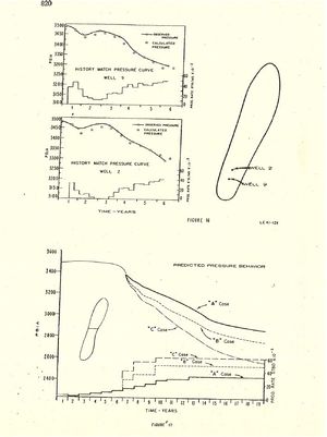
Figure 16 shows the quality of the pressure history Match for two individual wells. These plots, which are neither the best nor the poorest individual well plots, generally represent the behavior of the area. Figure 16 shows the pressure performance and location. of Wells No. 2 and 9. Well No. 2 has a maximum deviation from the observed pressure curve of 27 psi and an average deviation of about 10 psi. Well No. 9 has a maximum deviation from the observed pressure curve at one point of 35 psi; however, the average deviation is about 15 psi. For Well No. 9 the maximum deviation occurs early in the sixth year where the trend of the observed pressure values changes rapidly. This rapid change is due to a sharp cutback in production in the extreme southern end of the field. Figure 17 shows the predicted pressure behavior for 13 years for the three cases studied. The curve for Case "B" lies below the “A” case curve for all predicted time reflecting the greater pro¬duction rate used in the "B" case. At the end of prediction the “B” case curve lies about 83 psi below the "A" case curve. The curve for the "C" case lies below the "B" case curve throughout predicted time, reflecting The 10,000 barrel per day greater producing rate.

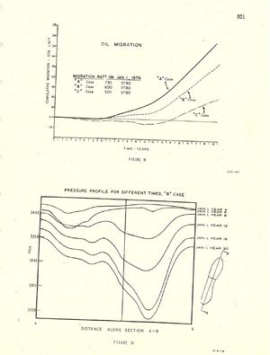
Figure 18 shows cumulative oil migration versus time for the three different production schedules and well placements. This migration is across the line bisecting the field shown in Figure 17.

Figure 19 shows the cause of the oil migration. The figure shows pressure profiles down the center of the field computed at different times for the "B" case. Similar plots could be obtained for the other two cases.

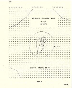
The regional isobaric map at the end of the prediction period for the "B" case is shown in Figure 20. This map, covering the entire model area, was generated by the IBM 7090 computer in about two minutes. For illustrative purposes, the field outline has been drawn on the map. The initial datum pressure was 3485 Asia every¬where. The radial behavior of the reservoir system is clearly shown by this map.

Nomenclature

A = total cross sectional area available to flow into and out of a tank
B = formation volume factor; relates reservoir volumes to standard volumes
Bg = gas formation volume factor
Bo = oil formation volume factor
Bw = water formation volume factor
c = compressibility; for tank model c = cR cv
cg = gas compressibility
co = oil compressibility
cR = rock compressibility